Privacy in databases

4. Privacy in databases#

4.1. Protecting Structured Data: From Tables to Queries#

Structured data, such as that collected in surveys or administrative databases, can often be transformed into tabular outputs for publication or analysis. Even aggregated tables, however, can leak sensitive information if small groups or unique combinations of attributes are disclosed. To mitigate this, statistical disclosure control (SDC) techniques modify or withhold risky cells.

Common SDC methods include:

Cell suppression, where small or sensitive counts are omitted, often with complementary suppression to prevent deduction from totals.
Controlled rounding or adjustment, which slightly modifies numerical values to obscure exact counts while preserving overall consistency.
Interval reporting, which replaces exact values with ranges (e.g., “between 3 and 7 cases”).
Noise addition, which introduces random perturbations calibrated to protect individual contributions.

The objective is to balance disclosure risk, i.e., the probability that an individual can be inferred, with information loss. Tabular data protection demonstrates that even aggregate statistics require careful anonymization to maintain confidentiality.

When users can query data directly, as in queryable databases, new risks arise. Repeated or overlapping queries can reconstruct individual information. To prevent this, systems employ:

Query restriction, refusing queries that affect too few records.

Query camouflage, returning generalized intervals instead of precise numbers.

Query perturbation, adding noise to query results.

The last approach leads to differential privacy (DP)—a formal framework ensuring that the inclusion or exclusion of any single individual’s data has negligible impact on the output. DP quantifies privacy through a parameter ε (epsilon): smaller ε means stronger protection but greater noise. Differential privacy has become a global standard, applied in government censuses and major technology platforms. Its conceptual ancestor, randomized response, introduced in the 1960s, uses randomness in survey answers to protect individuals while allowing valid statistical estimates—an intuitive early form of privacy-preserving data collection.

Microdata Anonymization

When individual-level data must be shared for research or statistical purposes, microdata anonymization transforms quasi-identifiers to prevent re-identification. The foundational model, k-anonymity, ensures that each record is indistinguishable from at least k–1 others. Extensions like l-diversity and t-closeness strengthen protection by maintaining diversity and distributional similarity in sensitive attributes, thus limiting attribute disclosure.

Anonymization methods can be:

Non-perturbative, preserving data correctness but reducing precision through generalization and suppression.

Perturbative, introducing controlled randomness (e.g., data swapping, noise addition, or synthetic data generation).

Risk–utility analysis guides the process: increasing privacy (higher k or tighter t) usually decreases analytical value, and the optimal balance depends on the use context. Microdata anonymization remains essential in health, social, and economic research, bridging classical statistical methods and modern privacy frameworks like differential privacy.

Privacy in Unstructured Data

Unstructured data—images, text, video, location traces, genomic sequences—poses unique challenges because identifiers are embedded in complex content rather than explicit fields.

For images, privacy risks arise from both content (faces, objects, backgrounds) and metadata (timestamps, GPS, device signatures). Common protections include blurring, pixelation, and masking, complemented by metadata cleaning. Newer methods use adversarial perturbations that fool face-recognition systems without perceptibly altering the image. In medicine, anonymization focuses on DICOM metadata removal and obscuring embedded text rather than modifying image content.

For textual data, privacy-enhancing NLP tools automatically detect and mask names, dates, and other sensitive terms using Named Entity Recognition (NER). Redaction can be performed by deletion or generalization; however, excessive sanitization may compromise semantic meaning. Synthetic text generation using large language models can provide an alternative by rewriting sensitive passages without reproducing original identifiers.

Location and genomic data pose especially high re-identification risks, as they are inherently unique. Location privacy is achieved through spatial and temporal generalization or the addition of noise, while genetic data typically relies on controlled access rather than anonymization, since true de-identification is infeasible.

Unstructured data anonymization thus combines content editing, metadata sanitization, and increasingly AI-assisted generation to balance privacy and utility in multimedia and textual information.

Privacy in Machine Learning

Machine learning systems amplify privacy challenges by processing vast, diverse datasets to extract predictive patterns. These models can unintentionally memorize or reveal sensitive data, creating new categories of attacks:

Membership inference attacks, which determine whether a given record was part of the training set.

Attribute inference, which deduces hidden features about individuals.

Model inversion and reconstruction, which regenerate approximate training examples.

Data poisoning, where malicious inputs alter the model or cause targeted leaks.

Mitigations span multiple layers:

Differentially Private Stochastic Gradient Descent (DP-SGD) injects noise during training to guarantee that model parameters reveal little about any single data point.

Federated learning keeps data local and aggregates updates across devices, often combined with secure aggregation and DP to prevent server-side inference.

Cryptographic computation (SMPC, homomorphic encryption) enables joint training or inference across institutions without sharing raw data.

Regularization and access control reduce overfitting and limit adversarial probing.

These approaches operationalize privacy by design in AI: models are trained and deployed under quantifiable privacy constraints rather than relying on post hoc anonymization.

Machine Unlearning and the Right to Be Forgotten

Privacy protection does not end when training concludes. Under the GDPR’s right to erasure, individuals may request that their data—and its influence—be removed from systems. Machine unlearning addresses this requirement by designing models capable of “forgetting” specific training samples efficiently, without full retraining.

Unlearning methods include:

Selective retraining, recomputing only affected components (e.g., trees in ensembles).

Influence-based rollback, estimating and reversing each record’s contribution to model parameters.

Gradient ascent unlearning, which counteracts the learned effect of deleted data.

Partitioned or modular training, designing models that can forget data partitions by design.

Certified unlearning frameworks aim to provide verifiable guarantees that a model behaves as if specific data were never used, bridging AI practice with legal accountability. This capability embodies the ultimate stage of privacy by design—systems that can both learn and forget responsibly.

Conclusion: The Continuum of Privacy by Design

Across these domains—structured, unstructured, and machine-learned data—the core challenge remains constant: balancing information utility with individual privacy. From risk assessment and anonymization to differential privacy and unlearning, each technique represents a step along a continuum from prevention to accountability.

Privacy by design is thus not a single technology but an ecosystem of principles, methods, and tools. It integrates cryptography, statistics, and artificial intelligence into a coherent discipline: privacy engineering. As data-driven systems grow more pervasive and autonomous, this discipline ensures that technological innovation remains aligned with ethical responsibility and human dignity.

Anonymization of structured databases is one of the central technical methods for protecting personal data while preserving its analytical or statistical value. Structured data, such as that stored in relational databases or spreadsheets, consists of well-defined attributes arranged in rows and columns—each row representing an individual and each column representing an attribute (such as age, income, or medical condition). These datasets are the foundation of much statistical, social, and biomedical research, yet they also pose serious privacy risks because individuals can often be identified or their attributes inferred, even after direct identifiers have been removed. The purpose of anonymization is to transform such data so that it can be used, published, or shared with third parties without revealing or allowing the inference of personal information.

To understand how anonymization works, it is essential to distinguish between different types of data attributes. Direct identifiers are attributes that uniquely identify a person on their own—such as a name, personal identification number, email address, or phone number. These are typically removed entirely in any anonymization process. Quasi-identifiers (or indirect identifiers) are attributes that do not identify an individual by themselves but can do so when combined with other information. Common examples include combinations of birth date, postal code, and gender, which have been shown to uniquely identify large portions of a population when cross-referenced with external data sources. Confidential attributes are those that are sensitive in nature, such as salary, medical diagnosis, or political opinion; these are not used to identify individuals but must be protected against disclosure. Finally, non-confidential attributes are those that carry little privacy risk and can typically be retained as-is.

When a dataset is released—either publicly or to specific researchers—the main risks are re-identification (linking data to an individual) and attribute disclosure (inferring confidential information about an identified person). These threats may arise from linkage attacks, in which an attacker combines anonymized data with external datasets, such as public voter registries or social media profiles, to re-establish identities. The well-known case of Latanya Sweeney’s re-identification of Massachusetts health records using public voter data illustrates this danger: even after names were removed, the combination of ZIP code, birth date, and sex uniquely identified a large percentage of individuals.

Structured data can appear in various forms depending on how it is shared. The simplest is tabular data, where aggregated statistics (like counts or averages) are published instead of individual records. While this reduces the risk of exposure, even aggregates can sometimes leak information when groups are small. Microdata releases contain individual-level records and pose higher risks but are more valuable for analysis. A third model involves queryable databases, where external users can run limited statistical queries without direct access to the data—an approach discussed more deeply in later sessions.

The core challenge of anonymization lies in finding the right balance between utility and privacy. If data is heavily modified or generalized, it may lose its usefulness for research or policy analysis; if it is insufficiently transformed, it remains vulnerable to privacy breaches. This balance can be described through two key measures: disclosure risk, the probability that an individual can be re-identified or a sensitive attribute inferred; and utility loss, the degree to which the anonymized data deviates from the original in ways that reduce its analytical value. In practice, anonymization often involves iterative processes that evaluate and adjust this trade-off.

Various approaches exist to anonymize structured data. A broad distinction can be made between non-perturbative and perturbative methods. Non-perturbative methods modify the structure of the data—by removing or grouping records, generalizing attribute values, or suppressing rare combinations—without changing the actual data values themselves. Examples include recoding numerical values into intervals (e.g., replacing exact ages with age ranges) or aggregating geographic details (replacing “street address” with “postal district”). Perturbative methods, on the other hand, introduce controlled randomness or noise to mask individual contributions while preserving global patterns. These include techniques like data swapping (exchanging values between records), noise addition (slightly altering numeric values), or synthetic data generation (creating artificial records that preserve statistical distributions).

To formalize privacy guarantees, researchers and practitioners use different models. The most widely known is k-anonymity, which requires that each record in a dataset be indistinguishable from at least k–1 others with respect to the quasi-identifiers. In other words, any given combination of identifying attributes must appear in at least k rows, making the probability of linking a record to a specific individual at most 1/k. Variants of this model, such as l-diversity and t-closeness, strengthen protection by ensuring diversity and similarity constraints within groups, reducing the risk of attribute disclosure even when sensitive attributes are unevenly distributed.

While these formal models are primarily applied to microdata, their principles also guide the anonymization of other data forms, including tabular and queryable data. In tabular data, cell suppression and controlled rounding are used to prevent inferences about small subgroups, while complementary suppression ensures that suppressed cells cannot be reconstructed from totals. When publishing frequency tables or census data, for instance, agencies routinely withhold or adjust values in small population groups to prevent re-identification.

An effective anonymization process typically begins with a detailed risk assessment. This includes identifying potential quasi-identifiers, estimating disclosure risk based on external data availability, and selecting appropriate transformation methods. After anonymization, utility evaluation ensures that the transformed data still supports the intended analyses—such as statistical inference, machine learning, or policy evaluation. Because anonymization is context-dependent, the same dataset might require different transformations depending on its intended use and audience: a public release requires stronger privacy, while restricted research access may allow more detail.

Ultimately, anonymization of structured databases illustrates a core theme in privacy engineering: privacy is not achieved by deleting data but by transforming it intelligently. It is a balance between protecting individuals and preserving collective knowledge. In practice, achieving full anonymity is nearly impossible—especially as external data sources multiply—but well-designed anonymization greatly reduces risk while maintaining social and scientific value.

4.2. Privacy in Databases#

An alternative strategy to protect data is to make them no longer linkable to individuals, that is, to anonymise them. Anonymised data are no longer considered personal, and thus the legal restrictions that apply to personal data are lifted. This section describes the state of the art in data anonymisation techniques and models.

4.2.1. Respondent Privacy: Statistical Disclosure Control#

Traditionally, national statistical institutes and government agencies have systematically gathered information about individual respondents, either people or companies, with the aim of using it for policymaking and also distributing it for public and private research that may benefit their country. The most detailed way to disseminate this information is by releasing a microdata set, essentially a database table, each of whose records conveys information on a particular respondent. Although these databases may be extremely useful to researchers, it is of fundamental importance that their publication does not compromise the respondents’ privacy in the sense of revealing information attributable to specific individuals. Statistical disclosure control (SDC) is the discipline that deals with the inherent trade-off between protecting the privacy of the respondents and ensuring that the protected data are still useful to researchers. Usually, a microdata set contains a set of attributes that may be classified as identifiers, key attributes (a.k.a. quasi-identifiers), or confidential attributes. Identifiers allow unequivocal identification of individuals. Examples are social security numbers or full names, which need to be removed before publication of the microdata set. On the other hand, key attributes are those attributes that, in combination, may allow linkage with external information to re-identify (some of) the respondents to whom (some of) the records in the microdata set refer (identity disclosure). Examples include job, address, age, gender, height and weight. Last but not least, the microdata set contains confidential attributes with sensitive information on respondents, such as salary, religion, political affiliation or health condition. Beyond protecting against identity disclosure, SDC must prevent intruders from guessing the confidential attribute values of specific respondents (attribute disclosure). Several SDC methods have been proposed in the literature to protect microdata sets (Hundepool et al. 2012). Next, we briefly review the main ones.

4.2.1.1. Non-perturbative Masking#

In SDC, masking refers to the process of obtaining an anonymised data set X’ by modifying the original X. Masking can be perturbative or non-perturbative. In the former approach, the data values of X are perturbed to obtain X’. In contrast, in nonperturbative masking X’ is obtained by removing some values and/or by making them more general; yet the information in X’ is still true, although less detailed; as an example, a value might be replaced by a range containing the original value. Common non-perturbative methods include:

Sampling. Instead of publishing the whole data set, only a sample of it is released.
Generalisation. The values of the different attributes are recoded in new, more general categories such that the information remains the same, albeit less specific.
Top/bottom coding. In line with the previous method, values above (resp. below) a certain threshold are grouped together into a single category.
Local suppression. If a combination of quasi-identifier values is shared by too few records, it may lead to re-identification. This method relies on replacing certain individual attribute values with missing values, so that the number of records sharing a particular combination of quasi-identifier values becomes larger.

4.2.1.2. Perturbative Masking#

Perturbative masking generates a modified version of the microdata set such that the privacy of the respondents is protected to a certain extent while simultaneously some statistical properties of the data are preserved. Well-known perturbative masking methods include:

Noise addition. This is the most popular method, which consists in adding a noise vector to each record in the data set. The utility preservation depends on the amount and the distribution of the noise.
Data swapping. This technique exchanges the values of the attributes randomly among individual records. Clearly, univariate distributions are preserved, but multivariate distributions may be substantially harmed unless swaps of very different values are ruled out.
Microaggregation. This groups similar records together and releases the average record of each group (Domingo-Ferrer and Mateo-Sanz 2002). The more similar the records in a group, the more data utility is preserved.

4.2.1.3. Synthetic Microdata Generation#

An anonymisation approach alternative to masking is synthetic data generation. That is, instead of modifying the original data set, a simulated data set is generated such that it preserves some properties of the original data set. The main advantage of synthetic data is that no respondent re-identification seems possible since the data are artificial. However, if, by chance, a synthetic record is very close to an original one, the respondent of the latter record will not feel safe when the former record is released. In addition, the utility of synthetic data sets is limited to preserving the statistical properties selected at the time of data synthesis. Some examples of synthetic generation include methods based on multiple imputation (Rubin 1993) and methods that preserve means and co-variances (Burridge 2003). An effective alternative to the drawbacks of purely synthetic data are hybrid data, which mix original and synthetic data and are therefore more flexible (Domingo-Ferrer and González-Nicolás 2010). Yet another alternative is partially synthetic data, whereby only the most sensitive original data values are replaced by synthetic values.

4.2.1.4. Privacy Models#

For an anonymised data set X’ to be safe/private enough, it needs to be sufficiently anonymised. The level of anonymisation can be assessed after the generation of X’ or prior to it. Ex post methods rely on the analysis of the output data set and, therefore, it is possible to generate a data set that is not safe enough according to a certain criterion; several iterations with increasingly strict privacy parameters and decreasing utility may be needed. The most commonly used ex post approach is masking followed by record linkage. Protection is sufficient high only if there is a sufficiently low proportion of masked records that can be linked to the respective original records they come from.

On the other hand, the ex ante approach relies on privacy models that allow selecting the desired privacy level before producing X’. In this way, the output data set is always as private as specified by the model, although it may fail to provide enough utility if the model parameters are too strict.

4.2.1.4.1. k-Anonymity and Extensions#

A well-known privacy model is k-anonymity (Samarati and Sweeney 1998), which requires that each tuple of key-attribute values be shared by at least k records in the database. This condition may be achieved through generalisation and suppression mechanisms, and also through microaggregation (Domingo-Ferrer and Torra 2005). Unfortunately, while this privacy model prevents identity disclosure, it may fail to protect against attribute disclosure. The definition of this privacy model establishes that complete re-identification is unfeasible within a group of records sharing the same tuple of perturbed key-attribute values. However, if the records in the group have the same value (or very similar values) for a confidential attribute, the confidential attribute value of an individual linkable to the group is leaked. To fix this problem, some extensions of k-anonymity have been proposed, the most popular being l-diversity (Machanavajjhala et al. 2006) and t-closeness (Li et al. 2007a). The property of l-diversity is satisfied if there are at least l ‘wellrepresented’ values for each confidential attribute in all groups sharing the values of the quasi-identifiers. The property of t-closeness is satisfied when the distance between the distribution of each confidential attribute within each group and the whole data set is no more than a threshold t.

4.2.1.4.2. Differential Privacy#

Another important privacy model is differential privacy (Dwork 2006). This model was originally defined for queryable databases and consists in perturbing the original query result of a database before outputting it. This may be viewed as equivalent to perturbing the original data and then computing the queries over the modified data. Thus, differential privacy can also be seen as a privacy model for microdata sets. An ε-differentially private algorithm is one that, when run on two datasets that differ in a single record, performs similarly (up to a power of ε) in both cases. That is, the presence or the absence of any single record does not significantly alter the output of the algorithm. Typically, ε-differential privacy is attained by adding Laplace noise with zero mean and parameter Δ(f)/ε, where Δ(f) is the sensitivity of the algorithm (the maximum change in the algorithm output that can be caused by a change in a single record in the absence of noise) and ε is a privacy parameter; the larger ε, the less privacy

4.3. Introduction#

In healthcare, data is often collected from patients to better understand disease patterns, improve treatments, and develop new medications. Some common types of data that are often used in biomedical research include: Demographic data: age, address, marital status, gender, etc. Social data: education, income, etc. Behavioral data: sleeping habits, smoker, drinker, drug user, etc. Clinical data: diagnostics, medications, test results, etc. Genomic data: genomic sequencing from samples. Image data: x-rays, CT-scans, MRI, fMRI, etc. Textual data: extra auxiliary information.

When processing, sharing, or releasing these data, we might do so as: Tabular data. Tables with counts or magnitudes. Queryable databases. On-line databases which accept statistical queries (sums, averages, max, min, etc.). Microdata. Files where each record contains information on an individual (a physical person or an organization).

Statistical databases must provide useful statistical information. They must also preserve the privacy of respondents if data are sensitive. Anonymization measures aim to produce modified versions of the original datasets which are as close as possible to the original datasets but do not allow attackers to identify individuals or to infer confidential attributes about specific individuals. Anonymous data are not classified as personal data and hence fall outside the scope of the GDPR.

Whichever the type and format of the data, the general aim of anonymization mechanisms is to minimize the risk of disclosure, in particular identity and/or attribute disclosure. In addition to accidental leakages, such disclosures can occur because of attacks. Record and attribute linkage attacks match auxiliary knowledge of an individual to records in private microdata sets to learn additional information about the target. Membership and attribute inference leverage released aggregate data, such as statistical tables or machine learning models, to improve their probabilistic belief in some piece of information about a target individual. Finally, reconstruction attacks try to reconstruct the original microdata (or training data in case of ML) from released statistics (or ML models).

Evaluation is in terms of two conflicting goals: Minimize the data utility loss caused by the method. Minimize the extant disclosure risk in the anonymized data. The best methods are those that optimize the trade-off between both goals. Two approaches exist to achieve this trade-off: Utility-first anonymization: apply masking methods iteratively until a desired disclosure risk is met. Privacy-first anonymization: use a privacy model, such as 𝑘-anonymity or 𝜖-differential privacy, which sets a disclosure risk, to derive parameters for masking methods.

4.4. Tabular data protection#

Tabular data is one of the most common ways in which statistical information is published. Government agencies, research institutions, and companies often release aggregated tables summarizing results from surveys, censuses, or databases—for example, the number of people by region and profession, or the average salary by sector. Although such tables appear harmless because they contain no individual records, they can still reveal sensitive information about individuals when analyzed carefully. Protecting privacy in tabular data publishing therefore requires specialized anonymization techniques that prevent both identity disclosure and attribute disclosure while maintaining the utility of the statistics.

A statistical table is usually constructed from microdata, meaning a collection of individual records that include multiple attributes for each person. When a table is built, those records are grouped according to certain key variables or quasi-identifiers (for example, region, age group, or gender), and a summary statistic—such as a count, total income, or average—is computed for each combination of categories. The resulting table thus contains cells, each representing a subgroup of individuals. For example, one cell might correspond to “Women aged 40–49 working in Finance in Barcelona.” Even though only the count or average is shown, if that subgroup includes very few individuals, those numbers could reveal private details about them.

Privacy risks in tabular data publishing can arise in two main ways. The first is the external attack: when an outside party uses publicly available information or background knowledge to deduce information about an individual. For instance, if a table reports that there is exactly one person in a specific region and category, an attacker who knows someone matching those conditions can infer that person’s confidential attribute (such as salary or health status). The second is the internal attack, which can occur even among respondents within the dataset. If two people appear in the same cell and one of them knows their own data, they can infer the other’s by comparing with the published cell value (for example, if they know the average salary of a two-person group and their own salary, they can deduce the other’s).

Because these risks depend on the number of individuals contributing to each cell, the cell frequency—the count of records behind each aggregate—is a crucial factor in tabular data protection. When cell frequencies are too small, the cell is considered unsafe. Statistical disclosure control (SDC) techniques aim to protect these cells while keeping the overall table as informative as possible.

The simplest protection strategy is cell suppression, where unsafe cells (those with very small counts or containing sensitive information) are removed or replaced with a symbol such as “–” or “confidential.” However, suppression alone can be insufficient because totals and marginal sums may allow suppressed values to be recalculated. To prevent such deductive disclosure, complementary suppression is applied: additional, non-sensitive cells are also suppressed strategically so that the missing values cannot be reconstructed from the published totals. This ensures that every suppressed cell is supported by a set of other suppressed cells that make re-computation impossible.

Another method is controlled rounding, in which numerical values—such as counts or averages—are rounded to the nearest multiple of a specified base (for example, to the nearest 3 or 5). Rounding introduces small random errors that obscure exact cell frequencies while preserving global consistency and additivity of totals. Controlled tabular adjustment (CTA) is a related approach that makes minimal adjustments to cell values, usually through optimization algorithms, to ensure that sensitive cells deviate from their true values by at least a specified threshold while keeping the table as close as possible to the original.

In some cases, agencies publish interval data rather than exact values. Instead of reporting an exact count or average, they publish ranges such as “between 3 and 7 individuals” or “average income between €35,000 and €40,000.” This technique generalizes results and can be tuned to balance privacy and precision: wider intervals give stronger privacy at the cost of utility.

Noise addition can also be applied to tabular data, though it must be done carefully to preserve statistical consistency. Small random perturbations are introduced to cell values or to the input data before aggregation, ensuring that the overall distribution remains accurate for analysis but that individual contributions cannot be deduced. However, because perturbation introduces distortion, it must be calibrated to maintain the credibility of published statistics—especially when the data serve policy or economic purposes.

To evaluate the effectiveness of these techniques, two criteria are commonly used: disclosure risk and information loss (or utility loss). Disclosure risk measures how likely it is that an individual’s information could be inferred from the published table. Information loss measures how much the modified table deviates from the original, affecting the usefulness of the data for analysis. An ideal anonymization strategy minimizes both—but in practice, they are inversely related: increasing protection typically reduces accuracy and vice versa. Agencies therefore aim for a reasonable balance based on the sensitivity of the data and the intended use of the publication.

In the practical workflow of tabular data protection, the process typically begins with identifying key variables—those attributes that could serve as quasi-identifiers—and determining a frequency threshold, such as three or five, below which a cell is considered unsafe. Then, one or more SDC methods (suppression, rounding, or perturbation) are applied. Finally, validation ensures that no suppressed or modified cells can be reconstructed through arithmetic relationships among totals or that noise addition does not excessively distort results.

An important aspect discussed in this session is that anonymizing tabular data is not the same as anonymizing microdata. In tabular data, individuals are already aggregated, so the primary goal is not to protect individual records directly but to prevent inference from aggregated statistics. The techniques, therefore, operate at the aggregate level—controlling how much information each published value reveals about the underlying data.

Ultimately, tabular data protection exemplifies one of the earliest and most classical forms of statistical disclosure control. It demonstrates the principle that even aggregate data can leak sensitive information if not handled carefully. By applying methods such as suppression, rounding, perturbation, and interval publication, data controllers can ensure that the results of statistical analyses remain useful for society while respecting the confidentiality of the individuals whose data underlie those numbers.

Goal: Publish static aggregate information, in such a way that no confidential information can be inferred on specific individuals to whom the table refers. From microdata, tabular data can be generated by crossing one or more categorical attributes. Formally, given categorical attributes $X_1, \cdots, X_l$, a table $T$ is a function $$T : D(X_1) \times D(X_2) \times \cdots \times D(X_l) \rightarrow R \; or \; N$$ where $D(X_i)$ is the domain where attribute $X_i$ takes its values.

4.4.1. Types of tables#

id	Salary	Sector	Region
1	500000€	IT	BCN
2	320000 €	IT	BCN
3	32000 €	IT	BCN
4	35000 €	IT	TGN
5	34000 €	IT	TGN
6	28000 €	IT	TGN
7	300000 €	HC	BCN
8	45000 €	HC	BCN
9	34000 €	HC	BCN
10	45000 €	HC	TGN
11	34000 €	HC	TGN
12	24000 €	HC	TGN
13	300000 €	Fin	BCN
14	350000 €	Fin	BCN
15	150000 €	Fin	TGN

Frequency	Region
Sector	BCN	TGN	Total
IT	3	3	6
Fin	2	1	3
HC	3	3	6
Total	8	7	15

Sum of Salary	Region
Sector	BCN	TGN	Total
IT	852000 €	97000 €	949000 €
Fin	335000 €	150000 €	485000 €
HC	379000 €	103000 €	482000 €
Total	1566000 €	350000 €	1916000 €

4.4.2. Disclosure attacks in tables#

External attack Let a released frequency table Ethnicity $\times$ Town contain a single respondent for ethnicity $E_i$ and town $T_j$. If a magnitude table is released with the average blood pressure for each ethnicity and each town, the exact blood pressure of the only respondent with ethnicity $𝐸_𝑖$ in town $𝑇_𝑗$ is publicly disclosed. Internal attack If there are only two respondents for ethnicity $𝐸_𝑖$ and town $𝑇_𝑗$ , the blood pressure of each of them is disclosed to the other. Dominance attack If one (or few) respondents dominate in the contribution to a cell in a magnitude table, the dominant respondent(s) can upper-bound the contributions of the rest. E.g., if the table displays the cumulative earnings for each job type and town, and one individual contributes 90% of a certain cell value, they know their colleagues in the town are not doing very well.

4.4.3. SDC Methods for tables#

Non-perturbative. They do not modify the values in the cells, but they may suppress or recode them. Best known methods: cell suppression (CS). recoding of categorical attributes. Perturbative. They modify the values in the cells. Best known methods: controlled rounding (CR). controlled tabular adjustment (CTA).

4.4.3.1. Cell suppression#

Identify sensitive cells, using a sensitivity rule. Suppress values in sensitive cells (primary suppressions). Perform additional suppressions (secondary suppressions) to prevent recovery of primary suppressions from row and/or column marginals.

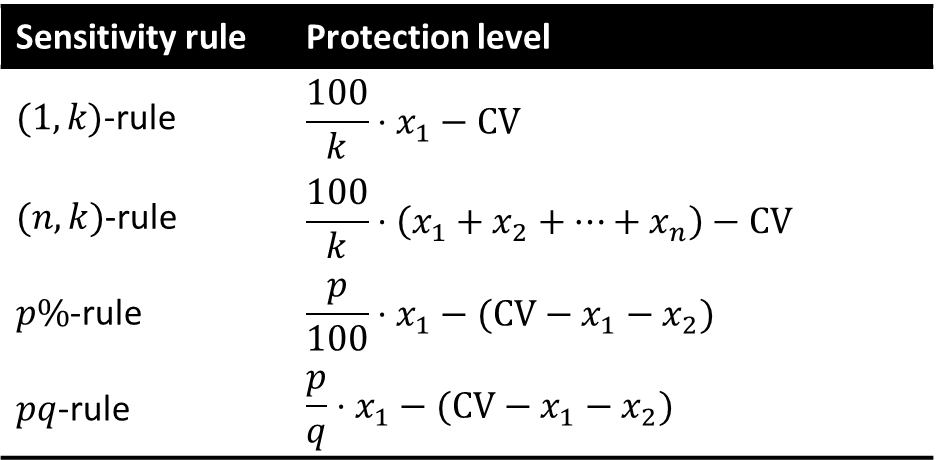
4.4.3.2. Sensitivity rules#

Minimum frequency rule: the cell frequency is less than a pre-specified minimum frequency 𝑛. (𝒏,𝒌)-dominance rule: the sum of the 𝑛 largest contributors exceeds 𝑘% of the cell total. 𝒑%-rule: the cell total minus the 2 biggest contributors is less than 𝑝% of the largest contribution. 𝒑𝒒-rule: Generalization of the 𝑝%-rule, which takes into account prior information. The 2nd biggest contributor can estimate the rest of contributions within 𝑞%.

Sum of Salary	Region
Sector	BCN	TGN	Total
IT	852000 €	97000 €	949000 €
Fin	335000 €	150000 €	485000 €
HC	379000 €	103000 €	482000 €
Total	1566000 €	350000 €	1916000 €

4.4.3.3. Secondary suppressions#

Usually, one attempts to minimize either the number of secondary suppressions or their marginals. Optimization methods are heuristic, based on mixed linear integer programming or networks flows (the latter for 2-D tables only).

Sum of Salary	Region
Sector	BCN	TGN	Total
IT	-	97000 €	949000 €
Fin	-	-	485000 €
HC	379000 €	103000 €	482000 €
Total	1566000 €	350000 €	1916000 €

A Feasibility Interval is the range of possible values that a suppressed cell can take, given the linear relations between cells and the row and column totals. In here, $X_{11}$ must be in range $[3,6]$, because $𝑋_{21}+𝑋_{22}= 3 \rightarrow 𝑋_{21} \le 3$, $𝑋_{11}+𝑋_{21}+3=9 \rightarrow 𝑋_{11} \le 6$, and $𝑋_{11}+𝑋_{21}+3=9 \rightarrow 𝑋_{11} \ge 3$.

Example	Attribute 1
Attribute 2	1	2	Total
1	X11	X12	7
2	X21	X22	3
3	3	3	6
Total	9	7	16

The feasibility interval must contain the protection interval. The protection interval is computed according to the chosen sensitivity rule $[𝐶𝑉−𝑃𝐿, 𝐶𝑉+𝑃𝐿]$.

alt text

4.4.3.4. Controlled rounding and Controlled tabular adjustment#

CR rounds values in the table to multiples of a rounding base (marginals may have to be rounded as well). CTA modifies the values in the table to prevent inference of sensitive cell values within a prescribed protection interval. CTA attempts to find the closest table to the original one that protects all sensitive cells. CTA optimization is typically based on mixed linear integer programming and entails less information loss than CS.

4.4.4. Utility loss in tabular SDC#

For cell suppression, utility loss is measured as the number of secondary suppressions or their pooled magnitude. For controlled tabular adjustment or rounding, it is measured as the sum of distances between true and perturbed cell values. The above loss measures may be weighted by cell costs, if not all cells have the same importance.

4.4.5. Disclosure risk in tabular SDC#

Disclosure risk is evaluated by computing the feasibility intervals for sensitive cells (via linear programming constrained by the marginals). What could be the range of values of the suppressed cells given other cells, including marginals? The table is safe if the feasibility interval for any sensitive cell contains the protection interval defined for that cell. If a cell was suppressed because of the 𝑝%-rule, does this 𝑝% lie within the feasibility interval? The protection interval is the narrowest interval estimate of the sensitive cell permitted by the data protector.

4.5. Interactive databases#

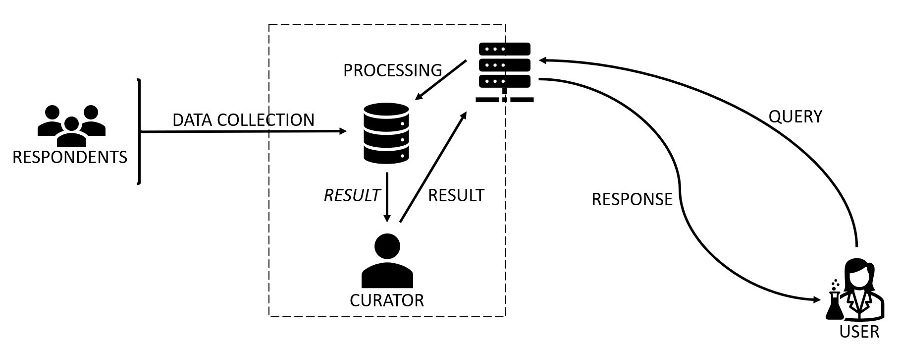
After discussing the protection of tabular data, which focuses on publishing static, aggregated statistics, this session turns to the more dynamic scenario of queryable databases—systems that do not publish raw or aggregated data directly but instead allow users to make statistical queries through controlled interfaces, such as APIs or query engines. These databases are increasingly common in government, research, and commercial environments because they promise flexibility: external analysts or applications can request statistics or summaries without the data ever leaving the controller’s server. However, this model still poses serious privacy challenges. Even when individual records are not exposed, the answers to queries can leak sensitive information, especially if users issue cleverly designed or repeated queries.

A queryable database typically consists of three entities:

A data controller or curator, who collects and stores data from respondents or participants (for example, through surveys, services, or sensors).

A dataset, often containing personal information, organized in relational form.

A user, who can submit statistical queries—such as counts, sums, or averages—via an interface, often programmatically.

The central privacy objective is to protect the respondents, not the users. That is, the system must ensure that queries cannot reveal confidential information about individuals whose data is stored in the database.

Privacy Risks in Queryable Databases

Even seemingly harmless queries can compromise privacy when their conditions isolate small subsets of individuals. For instance, if a query asks, “How many employees in the finance sector in Tarragona earn more than €100,000?” and the answer is “1,” an attacker might infer both the existence and the salary of that single individual. If follow-up queries refine conditions (for example, by changing filters or combining results), they can extract additional details. This risk increases when users collude or use external information to link responses with real-world identities.

Two main forms of disclosure can occur:

Identity disclosure, when a query indirectly reveals who an individual is.

Attribute disclosure, when the value of a confidential attribute (such as salary or diagnosis) can be inferred for an identified person.

Unlike static table publication, protecting a queryable database is an ongoing process: each new query potentially leaks more information. Thus, privacy protection mechanisms must monitor query patterns over time and enforce limits dynamically.

Three Families of Protection Techniques

Three broad strategies are used to protect queryable databases: query restriction, query camouflage (generalization), and query perturbation. Each offers a different balance between privacy, computational cost, and result accuracy.

Query Restriction The most straightforward method is to simply refuse to answer queries that could compromise privacy. The system computes the query set size—the number of individual records that match the query conditions—and denies responses when that number falls below a predefined threshold. For example, the system might only answer queries that affect at least three or five individuals. This prevents small-group disclosures and is analogous to cell suppression in tabular data.

The advantage of query restriction is that it preserves exact accuracy: all returned results are true and unmodified. However, it is extremely demanding to implement securely. The curator must not only monitor each query but also consider query history—because multiple queries can be combined to extract sensitive information even if each, individually, is safe. Keeping track of overlaps between query sets (and potential collusion between users) is computationally expensive, especially for large datasets or open systems with many users. Therefore, while conceptually simple, query restriction scales poorly in practice.

Query Camouflage (Interval or Generalized Responses) Another strategy is to generalize the answers by reporting intervals instead of precise values. For example, instead of returning that the average salary is €42,530, the system might report that it lies between €40,000 and €45,000. This method provides bounded uncertainty without adding random noise, which preserves logical consistency and allows unlimited querying.

Each confidential attribute can have its own privacy bound—a parameter defining how wide the intervals should be. A larger interval offers stronger privacy but reduces the utility of the data, since results become less specific. Because interval reporting does not distort the data but rather abstracts it, it is considered a non-perturbative method. However, as with other generalization approaches, it cannot fully prevent inference when users accumulate many queries with overlapping conditions.

Query Perturbation (Noise Addition) The most powerful and conceptually advanced approach is to add controlled noise to query responses so that individual contributions are hidden, while overall statistical patterns remain accurate. Noise can be introduced at two stages:

Input perturbation, where random noise is added to the raw data before any queries are processed.

Output perturbation, where noise is added to the query result itself before returning it to the user.

Input perturbation provides consistent privacy guarantees across queries but permanently modifies the dataset. Output perturbation preserves the dataset but requires generating new noise for each query, raising challenges for consistency and cumulative leakage.

Differential Privacy

The theoretical foundation for query perturbation is differential privacy (DP)—a mathematically rigorous model introduced in the mid-2000s and now widely used in both research and industry. Differential privacy formalizes the idea that the inclusion or exclusion of a single individual’s data should not significantly affect the result of any analysis.

More precisely, a randomized algorithm satisfies differential privacy if, for any two datasets that differ in only one individual, the probability of obtaining a particular output is nearly the same. The difference between these probabilities is controlled by a parameter called epsilon (ε), the privacy budget. A smaller ε provides stronger privacy (less sensitivity to any individual record) but introduces more noise and therefore reduces accuracy.

In practical terms, differential privacy gives a quantifiable, provable privacy guarantee that does not depend on what external information attackers might possess. It limits what can be inferred about any individual, even in the worst-case scenario. This makes it fundamentally stronger than heuristic approaches like suppression or generalization.

The implementation of differential privacy usually involves adding random noise drawn from a specific probability distribution—most commonly Laplace or Gaussian—to query outputs. The amount of noise depends on the sensitivity of the query function (how much a single individual’s data can change the result) and on the chosen privacy parameter ε. For example, a simple count query has sensitivity 1 (each individual can change the count by at most one), whereas averages or sums have higher sensitivity.

Differential privacy also introduces the concept of a privacy budget over multiple queries. Each query consumes part of the available ε; when the total budget is exhausted, no further queries can be answered without violating the overall privacy guarantee. This ensures that repeated querying cannot gradually erode privacy protection.

This model has become the de facto standard for privacy-preserving analytics. It has been adopted in high-profile deployments such as the U.S. Census Bureau’s 2020 census, which used differential privacy to protect published statistics, and by major technology companies like Apple, Google, and Meta for data collection and analysis of user behavior.

The Randomized Response Analogy

To make the intuition behind differential privacy more accessible, the lecture introduced an older statistical method called randomized response, developed in the 1960s for social science surveys. In randomized response, participants answer sensitive yes/no questions (for example, “Have you ever used illegal drugs?”) using a randomizing device such as a coin flip. If the coin lands heads, the respondent answers truthfully; if tails, they answer “yes” regardless of the truth. Because the interviewer cannot know whether any given answer is truthful, the individual’s privacy is protected. Yet, because the probability of randomness is known, the overall proportion of “yes” answers in the population can still be estimated statistically.

Differential privacy generalizes this idea to databases: by adding controlled randomness to query results, it protects individuals’ data while still allowing accurate aggregate statistics to be derived.

Conclusion

Queryable databases illustrate a fundamental trade-off between data utility and individual privacy. Restriction methods guarantee perfect accuracy but are computationally and operationally costly. Generalization provides deterministic uncertainty but can still be circumvented through repeated queries. Noise addition—especially as formalized by differential privacy—offers strong, quantifiable protection with manageable utility loss, making it the most promising modern approach.

This model marks a conceptual shift from heuristic anonymization toward mathematically provable privacy. Rather than focusing on hiding or deleting specific identifiers, differential privacy ensures that the participation of any individual has an almost negligible effect on analytical outcomes. It is, therefore, the cornerstone of contemporary privacy-preserving data analytics and the natural evolution of statistical disclosure control in the age of big data and machine learning

alt text

4.5.1. Issues#

id	Salary	Sector	Region
1	500000€	IT	BCN
2	320000 €	IT	BCN
3	32000 €	IT	BCN
4	35000 €	IT	TGN
5	34000 €	IT	TGN
6	28000 €	IT	TGN
7	300000 €	HC	BCN
8	45000 €	HC	BCN
9	34000 €	HC	BCN
10	45000 €	HC	TGN
11	34000 €	HC	TGN
12	24000 €	HC	TGN
13	300000 €	Fin	BCN
14	350000 €	Fin	BCN
15	150000 €	Fin	TGN

SELECT count() FROM table WHERE Salary > 100.000
Result = 5
SELECT sum(Salary) FROM table WHERE Sector = HC
Result = 482.000
SELECT count() FROM table WHERE Sector = IT and Region = TGN
Result = 3
SELECT count() FROM table WHERE Sector = Fin and Region = TGN
Result = 1
SELECT avg(Salary) FROM table WHERE Sector = Fin and Region = TGN
Result = 150.000

4.5.2. Interactive database protection#

Three main SDC approaches: Query restriction. The database refuses to answer certain queries. Camouflage. Deterministically correct non-exact answers (small interval answers) are returned by the database. Query perturbation. Perturbation (noise addition) can be applied to the microdata records on which queries are computed (input perturbation) or to the query result after computing it on the original data (output perturbation).

4.5.2.1. Query restriction#

This is the right approach if the user does require deterministically correct answers and these answers must be exact (i.e., a number). Exact answers may be very disclosive, so it may be necessary to refuse answering certain queries at some stage. A common criterion to decide whether a query can be answered is query set size control: the answer to a query is refused if this query together with the previously answered ones isolates too small a set of records. Problems: computational burden to keep track of previous queries, collusion possible.

4.5.2.2. Camouflage#

Interval answers are returned rather than point answers. No distortion of answers. Unlimited answers can be returned. Each query can only concern a single confidential attribute. Privacy bounds are set for each confidential attribute. The data curator can set a global bound, e.g., 30% (𝑢_𝑖−ℓ_𝑖≥0.3𝑥_𝑖). Respondents may request specific upper and lower bounds for their values.

4.5.2.3. Query perturbation#

Add noise to the values of confidential attributes in the original microdata (input perturbation). We will cover that when we talk about microdata protection. Add noise to the results of the queries after computing them on the original data (output perturbation). Under the differential privacy model, we can give theoretical guarantees on the privacy level achieved with output perturbation.

4.5.2.4. Randomized response#

There are $n$ people, and individual $i$ has a sensitive bit $X_i \in \{0,1\}$. Each person sends the analyst a message $Y_i$, which may depend on $X_i$ and some random numbers which the individual can generate. Based on these $Y_i$, the analyst would like to estimate $p=1/n \sum_i X_i$. Consider the following strategy, which we will call Randomized Response, parameterized by some $\gamma\in [0, 1/2]$. $Y_i = X_i$ with probability $1/2 + \gamma$ and $Y_i = 1-X_i$ with probability $1/2-\gamma$. How private $Y_i$ and how accurate will the estimation of $y$? It depends on $\gamma$. There is plausible deniability.

4.5.2.5. Differential privacy#

We imagine there are $n$ individuals, $X_1$ through $X_n$, who each have their own datapoint. They send this point to a “trusted curator”. Given their data, the curator runs an algorithm $M$, and publicly outputs the result of this computation. Differential privacy is a property of $M$ saying that no individual’s data has a large impact on the output. Suppose we have an algorithm $M:X^n \rightarrow Y$. Consider any two datasets $X, X' \in X^n$ which differ in exactly one entry. We call these neighboring datasets. We say that $M$ is $\epsilon$-differentially private ($\epsilon$-DP) if, for all neighboring $X, X'$, and all $T \subseteq Y$, we have $$Pr⁡[M(X) \in T] \le e^\epsilon Pr⁡[M(X') \in T]$$ where the randomness is over the choices made by $M$.

The sensitivity of a function $\Delta f$ (or $\Delta$ if $f$ is known) is the maximum distance between the results of $f$ computed on neighboring datasets. This can be defined as the $\ell_1$ distance between results of $M$ on neighboring datasets ($(\epsilon,\delta)$-DP requires the $\ell_2$ distance). For example:

Count queries have a $\Delta$ of 1.
Average queries have a $\Delta$ of $\max/n$.
Sum queries have a $\Delta$ of $\max$.

4.5.2.5.1. The Laplace mechanism#

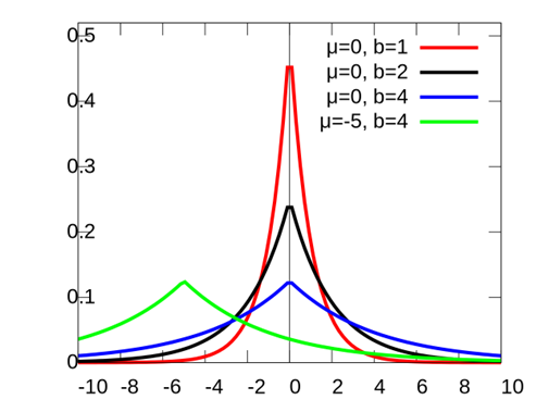
The Laplace mechanism is a fundamental technique for achieving differential privacy. Given a function $f: D \rightarrow R^d, where $D$ is the domain of the dataset and $d$ is the dimension of the output, the Laplace mechanism $M_{Laplace}$ adds Laplace noise to the output of $f$. That is $M_{Laplace}(D)=f(D)+Lap(\Delta/\epsilon)$ Let $b$ be the scale parameter of the Laplace distribution, which is given by: $$Lap(b)=\frac{1}{2b} e^{-\frac{|x|}{b}}$$

alt text

4.5.2.5.2. Properties of DP#

$\epsilon$ (privacy budget) should be small. Ideally in the range $(0,1]$. Resistance to post-processing. Once a quantity is privatized, it can’t be “un-privatized,” if the data is not used again. Group differential privacy. When neighboring datasets differ in $k$ positions, the guarantee goes to $k\epsilon-DP$. Composition rules. If we run $k$ $\epsilon_i$-DP algorithms on the same data, the privacy budget becomes $(\sum_{i=1}^k \epsilon_i)$-DP. We can assign a budget to each user.

4.5.3. Utility loss in interactive databases#

For query restriction, utility loss can be measured as the number of refused queries. For camouflage, utility loss is proportional to the width of the returned intervals. For query perturbation, the difference between the true query response and the perturbed query response is a measure of utility loss ⇒ this can be characterized in terms of the mean and variance of the noise being added (ideally, the mean should be zero and the variance small).

4.5.4. Disclosure risk in interactive databases#

In query restriction, the query set size below which queries are refused is a measure of disclosure risk (a query set size 1 means total disclosure). In camouflage, disclosure risk is inversely proportional to the interval width. If query perturbation is used according to a privacy model like $\epsilon$-differential privacy, disclosure risk is controlled a priori by the $\epsilon$ parameter (the lower, the less risk).

4.6. Microdata#

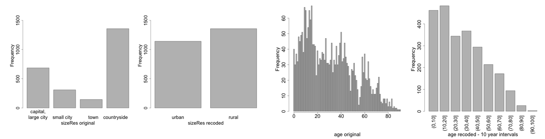
Microdata represents the most granular and detailed form of structured data: each record corresponds to an individual entity (a person, household, or organization), and each attribute describes some aspect of that entity—such as age, income, education, or health condition. Because microdata preserves individual-level information, it provides great analytical value for research and policymaking, but it also poses the highest privacy risks. Even after removing direct identifiers, individuals can often be re-identified by combining quasi-identifiers with external datasets. Microdata anonymization therefore seeks to transform such datasets to make re-identification or attribute inference practically impossible, while maintaining as much data utility as possible for statistical and analytical purposes.

Types of Attributes and Privacy Threats

As in previous discussions, attributes in microdata can be categorized into several classes:

Direct identifiers, such as name, ID number, or email, which uniquely identify an individual and must always be removed or masked.

Quasi-identifiers, which do not identify a person on their own but can do so in combination with other attributes (for example, age, ZIP code, and gender).

Confidential (or sensitive) attributes, which contain private information that should not be disclosed, such as salary, disease, or political affiliation.

Non-confidential attributes, which are neutral and generally harmless to share.

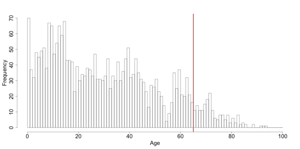
The main threats to privacy in microdata publication are re-identification (linking records to known individuals) and attribute disclosure (inferring sensitive information about an identified individual). These risks arise because even a few quasi-identifiers can uniquely characterize many people. A classic example is the discovery that 87% of Americans could be uniquely identified by the combination of ZIP code, gender, and date of birth.

Non-Perturbative vs. Perturbative Approaches

Anonymization methods for microdata are broadly divided into non-perturbative and perturbative techniques.

Non-perturbative methods preserve the truthfulness of data values but reduce their precision or granularity. This includes recoding, generalization, and suppression. For example, instead of publishing exact ages, data may be grouped into ranges (20–29, 30–39, etc.), or small geographic areas may be aggregated into larger regions. The idea is to ensure that each record becomes indistinguishable from several others with respect to the quasi-identifiers.

Perturbative methods, on the other hand, modify data values by introducing controlled randomness. This includes noise addition (slightly altering numerical values), data swapping (exchanging attribute values between records), rank swapping (reordering values among similar records), and synthetic data generation (creating entirely artificial records that preserve statistical distributions). These methods are particularly useful when precise micro-level accuracy is not required but overall statistical properties must remain valid.

Both categories aim to balance two competing objectives: minimizing disclosure risk and preserving analytical utility. The optimal choice depends on the purpose of the data release.

k-Anonymity: The Foundational Model

The most influential formal model for microdata anonymization is k-anonymity, introduced by Samarati and Sweeney in the late 1990s. A dataset satisfies k-anonymity if every combination of quasi-identifiers appears in at least k records. In other words, each individual is indistinguishable from at least k–1 others with respect to the identifying attributes. This means that the probability of correctly re-identifying any record is at most 1/k.

To achieve k-anonymity, the dataset is partitioned into equivalence classes, where each class contains at least k records that share the same generalized values for their quasi-identifiers. For example, if a dataset achieves 4-anonymity, each unique combination of age range, gender, and ZIP code must appear in at least four records. The process typically involves iterative generalization (grouping categorical values, widening numerical intervals) and suppression (removing overly unique records).

While k-anonymity provides a clear and intuitive privacy guarantee, it has limitations. It protects only against identity disclosure, not attribute disclosure. If all individuals in an equivalence class share the same value for a sensitive attribute—say, they all have the same medical diagnosis—then knowing that a person belongs to that group still reveals their confidential information. To address this, several stronger models were developed.

l-Diversity and t-Closeness: Beyond Identity Protection

l-Diversity extends k-anonymity by requiring that each equivalence class contain at least l well-represented values for every sensitive attribute. This ensures diversity within groups, reducing the risk of attribute disclosure. For instance, if an equivalence class of four records all indicate “HIV-positive,” the dataset is technically 4-anonymous but not diverse; an attacker would immediately learn that anyone in that group has HIV. Ensuring l-diversity means that sensitive attributes vary across the records in each group.

However, l-diversity can still fail when the overall distribution of a sensitive attribute is highly skewed. If one value (e.g., “flu”) dominates globally, then even a diverse group might not protect well. To address this, t-closeness was introduced. It requires that the distribution of a sensitive attribute within each equivalence class be close (within a distance t) to its distribution in the entire dataset. The smaller t is, the stronger the privacy guarantee. This model directly measures how much information about sensitive attributes can be inferred from group membership, ensuring that each group reflects the overall population distribution.

These models form a hierarchy of protection:

k-anonymity prevents identity disclosure.

l-diversity reduces attribute disclosure by ensuring variety.

t-closeness controls how much the internal distribution can deviate from the global one.

Practical Techniques: Masking and Recoding

In practical applications, microdata anonymization is often achieved through masking techniques that modify quasi-identifiers according to chosen privacy parameters. Common strategies include:

Global recoding, where values are replaced with broader categories (e.g., merging job titles into sectors).

Local suppression, where certain values are removed or replaced with missing entries in specific records that threaten anonymity.

Top- and bottom-coding, which cap extreme numerical values—for example, reporting all incomes above €200,000 simply as “≥200,000.”

Microaggregation, which replaces groups of similar records with group averages, commonly used for numerical data.

These transformations are carefully evaluated to ensure they maintain the statistical relationships necessary for analysis—such as means, variances, and correlations—while satisfying k-anonymity or its extensions.

Evaluating Risk and Utility

Every anonymization process involves measuring disclosure risk (the likelihood of re-identification) and information loss (the reduction in data quality or analytical power). Techniques such as risk–utility maps are used to visualize the trade-off between these two dimensions. Analysts can adjust parameters (e.g., the value of k or the granularity of generalization) to achieve the desired balance.

An additional consideration is the context of data release. For public data releases, stronger privacy (higher k or t) is required; for controlled research environments where access is restricted and monitored, weaker anonymization may suffice to retain utility.

Conceptual Transition: Toward Queryable and Differential Privacy

The anonymization of microdata bridges traditional statistical disclosure control and the more recent paradigm of differential privacy. While k-anonymity and its variants rely on modifying data before release, differential privacy introduces randomness during query processing. The former alters data values; the latter perturbs outputs. Both share the same goal—limiting how much information about any individual can be inferred—but differ in mathematical foundations and operational approach.

Microdata anonymization remains central in domains like healthcare, official statistics, and social research, where tabular or aggregate data is insufficient and researchers require individual-level information. It embodies the classic tension between privacy protection and scientific value, reminding us that the act of anonymization is not merely technical but also ethical: protecting individuals while preserving knowledge that can benefit society.

A microdata file $X$ with $s$ respondents and $t$ attributes is an $s \times t$ matrix where $X_{ij}$ is the value of attribute $j$ for respondent $i$.

alt text

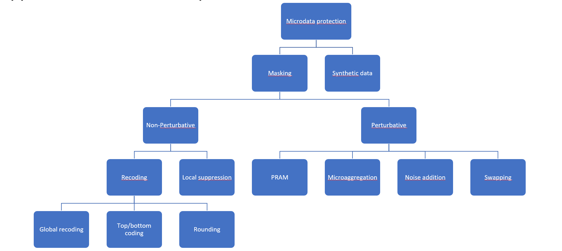
4.6.1. Non-perturbative masking#

4.6.1.1. Recoding#

Recoding is a non-perturbative, deterministic method for numeric and categorical attributes. Recoding is used to decrease the number of distinct categories or values for a variable. This is done by combining or grouping categories for categorical variables or constructing intervals for continuous variables. Recoding is applied to all observations of a certain variable and not only to those at risk of disclosure. There are two general types of recoding: global recoding and top and bottom coding.

4.6.1.1.1. Global recoding#

Global recoding combines several categories of a categorical variables or constructs intervals for continuous variables.

alt text

4.6.1.1.2. Top/bottom coding#

Top and bottom coding are similar to global recoding, but instead of recoding all values, only the top and/or bottom values of the distribution or categories are recoded.

alt text

4.6.1.1.3. Rounding#

Rounding is similar to grouping but used for continuous variables. Rounding is useful to prevent exact matching with external data sources. In addition, it can be used to reduce the level of detail in the data. Examples are removing decimal figures or rounding to the nearest 1,000.

4.6.1.2. Local suppression#

Certain values of individual attributes are suppressed to increase the set of records agreeing on a combination of quasi-identifier values. Recoding reduces the number of necessary suppressions as well as the computation time needed for suppression. Local suppression is not suitable for continuous variables or variables with a very high number of categories. A possible solution in those cases might be to first recode to produce fewer categories.

alt text

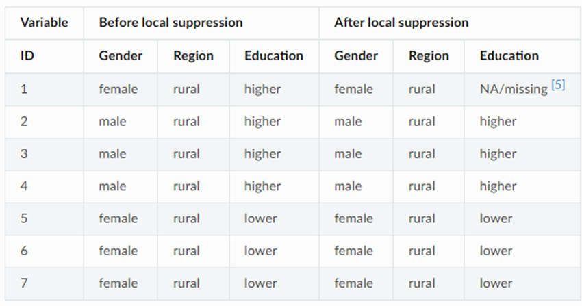
4.6.1.2.1. Recoding, suppression, and 𝑘-anonymity#

The computational approach originally proposed by Samarati and Sweeney to achieve 𝑘-anonymity combined recoding and suppression (the latter to reduce the need for the former). Most of the 𝑘-anonymity literature still relies on recoding, even though: Recoding cannot preserve the numerical semantics of continuous attributes. It uses a domain-level recoding hierarchy, rather than a data-driven one.

4.6.1.3. PRAM#

PRAM is a probabilistic perturbative method for categorical data. Each value of a categorical attribute is changed to a different value according to a prescribed Markov matrix (PRAM matrix). PRAM can afford transparency: publishing the PRAM matrix does not allow inverting anonymization. PRAM is useful when a dataset contains many variables and applying other anonymization methods would lead to significant information loss. A disadvantage of using PRAM is that very unlikely combinations can be generated.

4.6.1.4. Microaggregation#

Microaggregation is a statistical disclosure control technique that partitions a dataset into clusters of at least $k$ similar records according to their quasi-identifiers. Then, it replaces each cluster with a representative, such as the cluster centroid, to mask individual values. Consequently, each released record becomes indistinguishable from at least $k-1$ others, thus satisfying $k$-anonymity.

The Maximum Distance to Average Vector (MDAV) algorithm is a heuristic for $k$-anonymous microaggregation~\cite{domingo2002practical}. Given a dataset $X = \{x_1,\dots,x_n\} \subset \mathbb{R}^m$ with $n$ records consisting on $m$ quasi-identifier attributes, MDAV partitions $X$ into disjoint clusters of at least $k$ elements. Each record in a cluster is replaced by the cluster centroid, thus ensuring that each anonymized record is indistinguishable from at least $k-1$ others with respect to its quasi-identifiers~\cite{domingo2002practical}.

The algorithm works iteratively. At each step, the centroid $\bar{x}$ of the remaining records in $X$ is computed. The record $x_r$ that lies farthest from $\bar{x}$ is selected, and then the record $x_s$ that lies farthest from $x_r$ is chosen. A cluster is formed with $x_r$ and its $k-1$ nearest neighbors, and another with $x_s$ and its $k-1$ nearest neighbors. This process is repeated until fewer than $3k$ records remain. If the remaining number of records is between $2k$ and $3k$, they are split into two clusters; if it is less than $2k$, they form a single cluster.

Euclidean distance is typically used in the clustering phase, and the arithmetic mean of the records in each cluster is employed as the cluster representative value.

4.6.1.5. Noise addition#

Noise addition means adding or subtracting values to the original values of a variable and is most suited to protect continuous variables. Noise addition can prevent exact matching of continuous variables. The simplest version of noise addition is uncorrelated additive normally distributed noise $z_j=x_j+r_j$, where $r_j ~ N(0, \sigma_{r_j}^2)$ and $\sigma_{r_j} = \alpha \cdot \sigma_j$ If the level of noise added, $\alpha$, is disclosed to the user, many statistics can be consistently estimated from the perturbed data. Option: calibrate noise using $\epsilon$-differential privacy.

4.6.1.6. Swapping#

Data swapping was presented for databases containing only categorical attributes. Values of confidential attributes are exchanged among individual records, so that low-order frequency counts or marginals are maintained. Rank swapping is a variant of data swapping, also applicable to numerical attributes. Values of each attribute are ranked in ascending order and each value is swapped with another ranked value randomly chosen within a restricted range (e.g., the ranks of two swapped values cannot differ by more than 𝑝% of the total number of records).

4.6.2. Synthetic data generation#

Idea: Randomly generate data in such a way that some statistics or relationships of the original data set are preserved. Pros: No respondent re-identification seems possible, because data are synthetic. Cons: If a synthetic record matches by chance a respondent’s attributes, re-identification is likely and the respondent will find little comfort in the data being synthetic. Data utility of synthetic microdata is limited to the statistics and relationships pre-selected at the outset. Analyses on random subdomains are no longer preserved. Partially synthetic or hybrid data are more flexible.

4.6.3. Utility loss in microdata protection#

Data utility: Data use-specific utility loss measures. Generic utility loss measures. Disclosure risk: Fixed a priori by a privacy model: $\epsilon$-differential privacy, $k$-anonymity. Measured a posteriori by record linkage.

Number of suppressed records or values. Number of modified records. Means, variances, covariances, correlations… Distance metrics between original and anonymized datasets. Propensity score: The propensity score is a measure of indistinguishability between original and anonymized datasets. Merge the original and anonymized datasets and add a binary label $P$ with value $1$ for the anonymized records and $0$ for the original records. Predict $\hat{P}$, then $$U = 1 - \frac{1}{4} \sum_{i=1}^N \left( \hat{p}_i - \frac{1}{2} \right)^2$$

4.6.4. Disclosure risk in microdata protection#

4.6.4.1. A priori disclosure risk#

Using a privacy model like $k$-anonymity or differential privacy allows the tolerable disclosure risk to be selected at the outset. For $k$-anonymity the risk of identity disclosure is upper-bounded by $1/k$. $\epsilon$-Differential privacy can ensure a very low identity and disclosure (esp. for small $\epsilon$), but at the expense of a great utility loss.

A data set is said to satisfy $k$-anonymity if each combination of values of the quasi-identifier attributes in it is shared by at least $k$ records. A data set is said to satisfy $\ell$-diversity if, for each group of records sharing a combination of key attributes, there are at least $\ell$ “well-represented” values for each confidential attribute. A data set is said to satisfy $t$-closeness if, for each group of records sharing a combination of quasi-identifiers, the distance between the distribution of the confidential attribute in the group and the distribution of the attribute in the whole data set is no more than a threshold $t$.

4.6.4.2. A posteriori disclosure risk#

The uniqueness approach Typically used with non-perturbative masking. It measures disclosure risk as the probability that rare combinations of attribute values in the released data are indeed rare in the original population the data come from. The record linkage approach Attempt to link records between the anonymized and original records, either with perfect matches or with some distance measures. % of correct guesses → risk. It can be applied to any type of masking and synthetic data. It can even be applied to measure the actual disclosure risk of $\epsilon$-differentially private data releases.

4.6.5. Owner Privacy: Privacy-Preserving Data Mining#

Privacy-Preserving Data Mining (PPDM) tries to solve the following question: can we develop accurate data mining models without access to the data at the record level? Therefore, it consists of techniques for modifying the original data in such a way that the private data remain private even after the mining process (Verykios et al. 2004). There are two radically different approaches to PPDM, namely, PPDM based on perturbation and PPDM based on Secure Multiparty Computation (SMC). The first was introduced by Agrawal and Srikant (2000) in the database community. Its idea is that respondents (who do not wish to reveal the exact value of their respective answers/records) or controllers (who wish to engage in joint computation with other controllers without disclosing their respective data sets to each other) compute modified values for sensitive attributes in such a way that accurate statistical results can still be obtained on the modified data. PPDM based on perturbation is largely based on statistical disclosure control techniques. PPDM based on SMC, which was introduced by Lindell and Pinkas (2000) in the cryptographic community, addresses the problem of several entities holding confidential databases who wish to run a data mining algorithm on the union of their databases, without revealing unnecessary information. This type of PPDM is equivalent to data mining in distributed environments, where the data are partitioned across multiple parties. Partitioning can be vertical (each party holds all records on a different subset of attributes), horizontal (each party holds a subset of the records, but each record contains all attributes) or mixed. Using SMC protocols based on cryptography (many of these resort to homomorphic encryption) or on sharing perturbed information in ways that do not alter the final results often requires changing or adapting the data mining algorithms. Hence, each cryptographic PPDM protocol is designed for a specific data mining computation and, in general, is not valid for other computations. For example, a secure scalar product protocol based on cryptographic primitives is applied to privacy preserving k-means clustering over a distributed dataset by Vaidya and Clifton (2003) and Jagannathan and Wright (2005). Similarly, Du et al. (2004) and Karr et al. (2009) propose different ways (none of them based on encryption) to securely compute matrix products, which permits obtaining privacy-preserving linear regressions. A different PPDM scenario arises when a data controller wants to leverage the storage and also the computational power of untrusted clouds to process her sensitive data. This setting was studied in the H2020 project ‘CLARUS’ (http://clarussecure.eu) and solutions based on cleartext data splitting across several clouds have been proposed. Furthermore, protocols to compute scalar products and matrix products with minimum controller involvement and maximum cloud involvement have been given by Domingo-Ferrer et al. (2018).

4.6.6. User Privacy: Private Information Retrieval#

Finally, we address the privacy of the users querying a database. A history of queries to a database, or to a web search engine, can be used by the database owner to learn the interests of users, that is, to profile them. In this scenario, we seek to protect users from unrequested profiling by database owners. Mechanisms to achieve this goal are collectively referred to as private information retrieval (PIR). Initial works on PIR, such as Chor et al. (1995), model databases as vectors of entries. Users requesting information from the database do so by providing an index or a set of indices of the database vector. In this setting, PIR techniques aim to hide the indices provided by the users. However, these initial approaches have several shortcomings. First, they require collaboration from the database owner, something that cannot be ensured unless database owners have a clear incentive to do so. Second, to perfectly hide the queried database indices one would need to query all entries in the database and then filter the results locally, which is clearly inefficient for moderately sized databases and certainly unfeasible for big databases. Finally, modelling a database as a vector and assuming that the user knows the indices where the desired information is stored is not applicable to most real databases, let alone web search engines. Several solutions have been proposed to overcome such shortcomings. DomingoFerrer et al. (2009) propose a system named Goopir in which user queries are locally complemented with terms of similar frequency in the language (connected by OR operations). The responses are then filtered locally. TrackMeNot (Howe and Nissenbaum 2009) is a browser extension which periodically sends fake queries to web search engines so that the distribution of interests of the user is flattened and no useful profile can be extracted. Finally, other proposals such as the one by Reiter and Rubin (1998) make use of a P2P network in which users submit queries generated by other users to the web search engine, thus achieving the same results as TrackMeNot (flattened interest distributions) but without overloading the web search engines with fake queries.

4.7. (TEMP) Anonymization of Structured Databases#

4.8. Introduction#

In previous sessions we reviewed privacy-enhancing technologies for authentication, secure communication, and private computation. We now begin a three-week block dedicated to the anonymization of structured databases, which is one of the central technical approaches for publishing or sharing data while preserving individual privacy. Structured data refers to information stored in well-defined relational tables or spreadsheets, where each row corresponds to an individual and each column to an attribute. The purpose of anonymization in this context is to transform data so that it continues to provide useful statistical information while significantly reducing the risk that individuals can be re-identified or that confidential information about them can be inferred. When anonymization is carried out properly and linkability is broken, the resulting data is no longer considered personal data under the GDPR, although debates remain about what counts as “proper anonymization.”

4.9. Types of Data#

From a semantic perspective, structured data may include demographic information such as age or marital status, socioeconomic characteristics such as education and income, behavioural information describing habits or mobility patterns, and clinical or medical information such as diagnoses or treatments. Beyond these, there exist unstructured forms of data, such as text, images, genomic sequences, GPS traces, that will be addressed separately.

The same dataset can also be classified by the type of data values it contains. Numeric data includes integers or real-valued measurements associated with individuals. Categorical data may be ordinal when categories follow a meaningful order, or nominal when categories have no order at all.

Finally, structured data can be classified by its relevance to identifiability and sensitivity. Direct identifiers, such as names or phone numbers, uniquely identify individuals and are normally removed before any release. Quasi-identifiers, such as age, gender, or postal codes, do not identify a person on their own but can do so when combined with additional information. Confidential attributes include sensitive information that should not be disclosed, such as salary or medical conditions. Some attributes serve administrative purposes and carry no sensitive meaning; these are considered non-confidential.

4.10. Types of Tables for Release#

Organizations generally release structured data in three forms. Tabular data consists of static tables where each cell contains an aggregated count or numerical value. Queryable databases provide a controlled interface that allows users to perform statistical queries without exposing underlying individual records. Microdata releases, which provide one row per individual record, are the most detailed and sensitive.

4.11. Utility vs. Disclosure Risk#

Any anonymization procedure must balance two competing goals: preserving the usefulness of the released data and reducing the privacy risks associated with its disclosure. Utility loss measures how much statistical value is diminished by the anonymization process, while disclosure risk measures how much potential remains for re-identification or the inference of sensitive information. There are two general approaches to achieving this balance. In the utility-first approach, disclosure risk is estimated empirically—often by performing simulated attacks—and anonymization is progressively applied until risk falls below an acceptable level. In the privacy-first approach, theoretical privacy models such as k-anonymity or differential privacy are used to set target privacy parameters at the outset, and transformations are then chosen to meet those requirements.

4.12. Tabular Data: Frequency and Magnitude Tables#

Tabular releases are usually derived from an internal microdata file. For example, a dataset containing attributes such as salary, sector, and region can be transformed into a frequency table that counts how many individuals fall into each (sector × region) combination. Similarly, a magnitude table can be created in which each cell contains the sum, average, or another statistical compilation of a confidential attribute, such as salaries. These tables typically retain row totals, column totals, and grand totals, since such marginal information is often essential for statistical use.

4.12.1. Attacks on Tabular Data#

Although aggregated, these tables may leak private information through several mechanisms. External attacks occur when only one person contributes to a cell, making their confidential value immediately exposed if a magnitude table is available. Internal attacks arise when exactly two contributors are present; in such cases each one can infer the other’s contribution by subtracting their own from the aggregate. Dominance attacks occur when one or a few individuals heavily influence a magnitude cell, permitting inferences about their confidential values even when the cell contains three or more people.

4.12.2. Protection Methods#

Methods for protecting tabular data may be non-perturbative or perturbative. Non-perturbative techniques do not distort the values but limit their detail. The most common method is cell suppression, which removes values from sensitive cells. Another non-perturbative option is recoding the categories of the attributes—such as merging similar regions or sectors—so that more individuals fall into each cell and sensitivity is reduced.

Perturbative methods, in contrast, alter values directly. Controlled rounding modifies each cell to the nearest multiple of a chosen base, and controlled tabular adjustment uses linear optimisation to redistribute values while preserving the row and column totals. These perturbative approaches may be unsuitable in high-stakes environments, such as healthcare, where analysts rely on precise information.

4.12.3. Cell Suppression in Detail#

Cell suppression proceeds in two stages. The first stage, primary suppression, begins by identifying sensitive cells using predefined sensitivity rules. One such rule is the minimum frequency rule, which requires a cell to contain at least a certain number of contributors—commonly three—to avoid the risks associated with external or internal attacks. The next set of rules concerns dominance. Under the NK dominance rule, a cell is considered unsafe when the largest contributors account for more than a specified percentage of the total. The p-percent rule identifies a cell as unsafe when the contributions from all but the largest contributors fall below a certain fraction of the total. Once these sensitive cells are identified, their values are removed from the table.

However, after such suppressions, the remaining published structure—especially row and column totals—may enable someone to reconstruct the missing values. This need for protection leads to the second stage, secondary suppression, in which additional non-sensitive cells are removed to prevent such reconstruction. Determining which additional cells to suppress requires computing feasibility intervals. A feasibility interval expresses the range of possible values a suppressed cell may take while satisfying all the linear constraints imposed by the table’s totals. These intervals are compared to protection intervals that are derived from the sensitivity rules themselves. A table is considered safe once every protection interval is fully contained within its corresponding feasibility interval, meaning no sensitive value can be inferred too precisely.

4.12.4. Utility and Risk Evaluation#

The quality of anonymization is assessed by examining both utility loss and residual disclosure risk. Utility loss in the context of cell suppression can be measured by the number of suppressed cells or the sum of their magnitudes. In perturbative methods, utility may be measured by the differences between the original and adjusted cell values. Disclosure risk is quantified by analysing how well the feasibility intervals shield the sensitive cells given the protection intervals. The chosen sensitivity rules effectively define the acceptable level of disclosure risk.

4.12.5. Real-World Use#

These anonymization techniques are widely used in practice. European statistical agencies, including Eurostat and national statistics offices such as that of the Netherlands, routinely apply minimum frequency rules and cell suppression to protect published regional tables. Software for suppressing tabular data, including tools developed through European research projects, incorporates the techniques discussed here. In the United States, the Census Bureau historically relied on methods such as data swapping but has recently transitioned to differential privacy to protect the underlying microdata before constructing published tables. This shift has sparked discussions about accuracy, fairness, and the impact on small or under-represented groups, illustrating the broader consequences of anonymization choices.

4.13. Interactive Statistical Databases#

The previous discussion focused on anonymizing static tabular data. Another common scenario arises when organizations do not publish the data itself but instead provide a statistical interface through which external users can query aggregated information. These systems are known as interactive statistical databases. In this setting, the data remains with a curator or data controller, who collects information from respondents and stores it, while external users or analysts issue queries through an API. The curator receives the query, computes the requested statistic on the underlying microdata, and returns the result, possibly after applying privacy-preserving transformations.

alt text

Typical queries include counts, sums, averages, variances, and combinations of categorical selections, much like SQL queries. For example, one may query how many individuals in the database earn over a certain salary threshold, or the total salary paid to all workers in a particular sector, or the number of employees in a given region and industry. These are straightforward computations, but when the conditions defining the subset are too specific, the result may correspond to only one individual or a small number of them. In that case, returning the exact aggregate value would reveal sensitive information, including the confidential attributes of identified persons.

id	Salary	Sector	Region
1	500000€	IT	BCN
2	320000 €	IT	BCN
3	32000 €	IT	BCN
4	35000 €	IT	TGN
5	34000 €	IT	TGN
6	28000 €	IT	TGN
7	300000 €	HC	BCN
8	45000 €	HC	BCN
9	34000 €	HC	BCN
10	45000 €	HC	TGN
11	34000 €	HC	TGN
12	24000 €	HC	TGN
13	300000 €	Fin	BCN
14	350000 €	Fin	BCN
15	150000 €	Fin	TGN

SELECT count() FROM table WHERE Salary > 100.000
Result = 5
SELECT sum(Salary) FROM table WHERE Sector = HC
Result = 482.000
SELECT count() FROM table WHERE Sector = IT and Region = TGN
Result = 3
SELECT count() FROM table WHERE Sector = Fin and Region = TGN
Result = 1
SELECT avg(Salary) FROM table WHERE Sector = Fin and Region = TGN
Result = 150.000

This vulnerability leads to attacks analogous to those discussed for tabular data. If a query returns a count of one, the confidential attributes of that one respondent may be inferred. Even if counts are larger, cleverly constructed combinations of queries can enable difference attacks, where an attacker issues two overlapping queries and subtracts the results to isolate the contribution of one person. Such attacks exploit the interactive nature of the system: each result, even if individually harmless, may reveal information when combined with others.

4.14. Approaches to Protecting Interactive Queries#

Three broad strategies emerge for mitigating disclosure risk in interactive databases: query restriction, output generalization through intervals, and query perturbation.

Query restriction involves refusing to answer queries that would reveal too much information. The curator monitors the set of respondents affected by each query—its query set size—and ensures that it always exceeds some threshold. The difficulty is that disclosure risk depends not only on the current query but also on previous queries. To decide whether a new query is safe, the curator must track the cumulative information the user has already learned, which is computationally expensive and practically unmanageable. While query restriction guarantees correct, unmodified results for all answered queries, the method becomes infeasible at scale because of the need to track large query histories and to guard against collusion or multiple coordinated users.

A second approach is to provide generalized outputs: instead of returning exact numerical answers, the system returns intervals. This mirrors the idea of generalization in microdata anonymization, but applied to query results. For example, instead of stating that the average salary in a subset is 42,000€, the system might respond that it lies between 35,000€ and 50,000€. The width of the interval can be configured based on the desired privacy–utility trade-off. Wider intervals offer stronger privacy but reduce analytical precision. A key advantage is that queries can be answered without noise, and users can submit an unlimited number of queries, but the cost is reduced accuracy. The method becomes less effective when analysts require precise estimates or when multiple confidential attributes are involved.

The third and most general approach is query perturbation, in which the curator modifies the result before returning it, usually by adding noise. This can be done either via input perturbation, where noise is added to the underlying data before any queries are answered, or output perturbation, where each query result is computed exactly and then noise is added. Output perturbation is the more flexible and widely used variant because it allows the curator to tailor the magnitude of noise to each specific query.

4.14.1. Randomized Response as an Intuition#

To introduce the rationale behind query perturbation, it is helpful to consider randomized response, a classical technique from the 1960s for conducting surveys on sensitive topics. Respondents might refuse to answer questions about drug use, sexual behavior, or other stigmatized activities, or they might lie. Randomized response provides respondents with plausible deniability by instructing them to randomize their answers according to a known protocol. For example, each person may flip a private coin: with probability (1/2 + \gamma), they answer truthfully; with probability (1/2 - \gamma), they lie and report the opposite. A researcher who knows the value of (\gamma) can estimate the true proportion of “yes” responses in the population, while no outsider can confidently determine any individual’s truthful answer because the respondent can always claim that the randomization dictated their response.

When (\gamma = 0), the respondent answers truthfully half the time and lies half the time, so the responses contain almost no usable signal. When (\gamma = 1/2), respondents always tell the truth, which yields perfect utility but no privacy. Values in between provide a controllable trade-off between individual privacy and statistical accuracy. This balance serves as an intuition for the more formal framework of differential privacy.

4.14.2. Toward Differential Privacy#

Randomized response corresponds to a “local” privacy model, where individuals apply noise themselves. Differential privacy instead assumes that respondents provide their true data to a trusted curator, who stores all individual records and receives queries from external analysts. The goal is for the curator to answer analytics queries in a way that protects each respondent’s privacy, regardless of an analyst’s auxiliary knowledge or computational power.

The key idea is that the output of any analysis should not change too much when the data of a single individual is added or removed. To formalize this, we consider neighboring datasets—datasets that differ in exactly one individual’s record. A differentially private algorithm ensures that the probability of producing any given output changes only slightly between neighboring datasets. This stability guarantees that no analyst can confidently infer whether a particular individual contributed to the dataset.

$\epsilon$-Differential privacy

Differential privacy is a property of $M$ saying that no individual’s data has a large impact on the output. Suppose we have an algorithm $M:X^n \rightarrow Y$. Consider any two datasets $X, X' \in X^n$ which differ in exactly one entry. We call these neighboring datasets. We say that $M$ is $\epsilon$-differentially private ($\epsilon$-DP) if, for all neighboring $X, X'$, and all $T \subseteq Y$, we have

\[Pr⁡[M(X) \in T] \le e^\epsilon Pr⁡[M(X') \in T]\]

where the randomness is over the choices made by $M$.

To determine how much noise must be added to a query, one must compute its sensitivity: the maximum possible change in the query’s output when applied to neighboring datasets. For count queries, the sensitivity is 1, because removing or adding a single record changes the count by at most one. For averages, the sensitivity depends on the range of the attribute and the number of individuals included. For sums, the sensitivity equals the maximum possible value of the confidential attribute (for example, using an upper bound on age or salary). Bounding sensitivity is essential because differential privacy mechanisms calibrate their noise to this value.

The sensitivity of a function $\Delta f$ (or $\Delta$ if $f$ is known) is the maximum distance between the results of $f$ computed on neighboring datasets. This can be defined as the $\ell_1$ distance between results of $M$ on neighboring datasets ($(\epsilon,\delta)$-DP requires the $\ell_2$ distance). For example:

Count queries have a $\Delta$ of 1.
Average queries have a $\Delta$ of $\max/n$.
Sum queries have a $\Delta$ of $\max$.

One widely used mechanism for ensuring differential privacy is the Laplace mechanism, which adds noise drawn from the Laplace distribution. The scale of the Laplace distribution is proportional to the ratio of the query’s sensitivity to the privacy parameter $\epsilon$. Larger $\epsilon$ allows less noise and weaker privacy; smaller $\epsilon$ requires more noise and yields stronger privacy. Graphically, decreasing noise corresponds to a sharply peaked distribution around zero, while increasing noise yields a broader distribution. By adjusting $\epsilon$, practitioners can tune the privacy–utility trade-off: more privacy requires more noise, and therefore less statistical accuracy.

The Laplace Mechanism

The Laplace mechanism is a fundamental technique for achieving differential privacy. Given a function $f: D \rightarrow R^d$, where $D$ is the domain of the dataset and $d$ is the dimension of the output, the Laplace mechanism $M_{Laplace}$ adds Laplace noise to the output of $f$. That is $M_{Laplace}(D)=f(D)+Lap(\Delta/\epsilon)$ Let $b$ be the scale parameter of the Laplace distribution, which is given by: $$Lap(b)=\frac{1}{2b} e^{-\frac{|x|}{b}}$$

alt text

4.14.3. The Privacy Budget and Repeated Queries#

Each differentially private response consumes a portion of a privacy budget. Because answering queries reveals information, even noisy answers accumulate privacy loss. Differential privacy provides composition theorems that quantify how privacy degrades across multiple queries. In practice, curators limit the total number of queries or allocate budget portions to maintain global privacy guarantees.

This model addresses the primary weaknesses of earlier approaches. It does not rely on tracking overlapping query sets, does not prevent analysts from issuing many queries, and works even when attackers have extensive external knowledge. Instead, it provides mathematically provable guarantees that no single respondent’s data can be detected from the outputs, while still allowing analysts to extract meaningful aggregate information.

Privacy in databases

Contents

4. Privacy in databases#

4.1. Protecting Structured Data: From Tables to Queries#

4.2. Privacy in Databases#

4.2.1. Respondent Privacy: Statistical Disclosure Control#

4.2.1.1. Non-perturbative Masking#

4.2.1.2. Perturbative Masking#

4.2.1.3. Synthetic Microdata Generation#

4.2.1.4. Privacy Models#

4.2.1.4.1. k-Anonymity and Extensions#

4.2.1.4.2. Differential Privacy#

4.3. Introduction#

4.4. Tabular data protection#

4.4.1. Types of tables#

4.4.2. Disclosure attacks in tables#

4.4.3. SDC Methods for tables#

4.4.3.1. Cell suppression#

4.4.3.2. Sensitivity rules#

4.4.3.3. Secondary suppressions#

4.4.3.4. Controlled rounding and Controlled tabular adjustment#

4.4.4. Utility loss in tabular SDC#

4.4.5. Disclosure risk in tabular SDC#

4.5. Interactive databases#

4.5.1. Issues#

4.5.2. Interactive database protection#

4.5.2.1. Query restriction#

4.5.2.2. Camouflage#

4.5.2.3. Query perturbation#

4.5.2.4. Randomized response#

4.5.2.5. Differential privacy#

4.5.2.5.1. The Laplace mechanism#

4.5.2.5.2. Properties of DP#

4.5.3. Utility loss in interactive databases#

4.5.4. Disclosure risk in interactive databases#

4.6. Microdata#

4.6.1. Non-perturbative masking#

4.6.1.1. Recoding#

4.6.1.1.1. Global recoding#

4.6.1.1.2. Top/bottom coding#

4.6.1.1.3. Rounding#

4.6.1.2. Local suppression#

4.6.1.2.1. Recoding, suppression, and 𝑘-anonymity#

4.6.1.3. PRAM#

4.6.1.4. Microaggregation#

4.6.1.5. Noise addition#

4.6.1.6. Swapping#

4.6.2. Synthetic data generation#

4.6.3. Utility loss in microdata protection#

4.6.4. Disclosure risk in microdata protection#

4.6.4.1. A priori disclosure risk#

4.6.4.2. A posteriori disclosure risk#

4.6.5. Owner Privacy: Privacy-Preserving Data Mining#

4.6.6. User Privacy: Private Information Retrieval#

4.7. (TEMP) Anonymization of Structured Databases#

4.8. Introduction#

4.9. Types of Data#

4.10. Types of Tables for Release#

4.11. Utility vs. Disclosure Risk#

4.12. Tabular Data: Frequency and Magnitude Tables#

4.12.1. Attacks on Tabular Data#

4.12.2. Protection Methods#

4.12.3. Cell Suppression in Detail#

4.12.4. Utility and Risk Evaluation#

4.12.5. Real-World Use#

4.13. Interactive Statistical Databases#

4.14. Approaches to Protecting Interactive Queries#

4.14.1. Randomized Response as an Intuition#

4.14.2. Toward Differential Privacy#

4.14.3. The Privacy Budget and Repeated Queries#